\[ \]

Integration

Issue No 50, 6 November 2023

By: Anthony O. Ives

In the most simple terms integration is the reverse of differentiation [1], for example you should now be familar with the linear equation [2], therefore if you the know the rate of change of one varible against another variable, using integration you should be able return to the orginal linear equation if your rate of change is constant. However, another use for integration is that it can used to determine areas confined by a curve or set of curves. If you know the exact mathematical equation of the curve you can calculate an exact area if the equation is not known or is difficult to integrate then numerical integration can be used to estimate the area. Numerical integration can be performed using simpson's rule. For the present we will look at exact integration methods and look at simpson's rule in a later article.

As explained with differentiation an obvious example of rate of change is velocity which is rate of change of distance with respect to time, so therefore if you know an mathematical expression for velocity then you can integrate it with respect to time to give you a expression which can be used to calculate the distance travelled within a certain time. As with I did with differentiation, it applies to any two variables which there is a relationship between, so in the rest of the article I use general terms and refer to variable y the dependent variable and x the independent variable but if you get confused just compare them to distance and time which you can then relate to speed and acceleration.

As with differenatiation there are standard expressions for wide range of mathematical functions but we will start with the common one which is polynomial functions therefore if:

\[y = x^n\] Then: \[ \int_{a}^{b} x^n \,dx = \left[\frac{1}{n+1} x^{n+1} \right]_{a}^{b}\] or: \[ \int x^n \,dx = \frac{1}{n+1} x^{n+1} + C\]

If you remember from differentiation [1], when you differentiate the linear equation constants just simply disappear. Therefore when you integrate which as explained is the reverse of differentiation then you must reinstate the constant, but you do not know the constant so intially you can represent it as 'C' or some other appropiate symbol. In order to detemine the constant you would have to know some boundary conditions, if you take speed, distance and time as example then you might know the distance you started at. However, you could also use limits, using speed, distance, time again as example after integrating your speed and getting an expression for distance simply calcuation for a time 'a' and a time 'b' and subtract the one distance from another this would simply cancel out the constant but give you the distance travelled between times 'a' and 'b'. Below I will demonstrate integration using the linear equation as example.

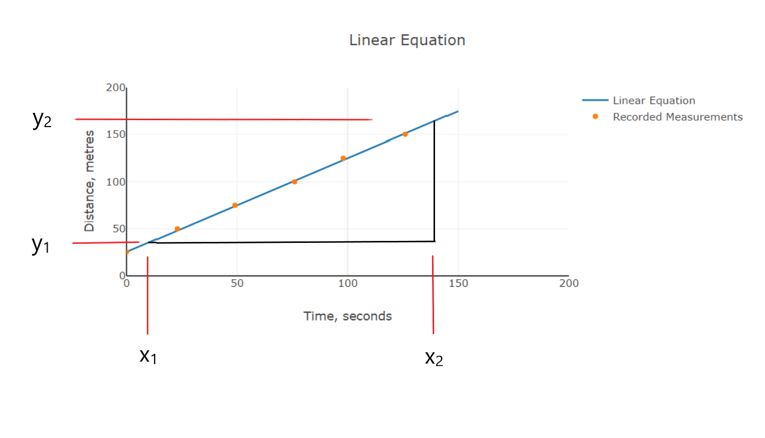
If you remember the gradient of the linear equation [1] is a constant value usually represented as 'm': \[ \frac{dy}{dx} = m\] Where m is known as the gradient see the picture below:

Linear Equation drawn on a Graph

Therefore integrating this constant value gives the linear equation:

\[y = \int mx^0 \,dx\] \[y = \frac{1}{0+1}mx^(0+1) +c \] \[y = mx + c\]

However, if we do the example using limits:

\[y = \int_{a}^{b} mx^0 \,dx\] \[y = \left[ \frac{1}{0+1}mx^(0+1) \right]_{a}^{b} \] \[y = (mb + c) - (ma + c)\] \[y = m(b-a)\]

So as explained the constant term cancels out so you are calculating the change in y from when x=a to when x=b. As a further example of integration you can use it to determine the quadratic equation from a linear equation using the same example as we did with differentiation:

\[ \frac{dy}{dx} = 2x + 7\] \[y = \int 2x + 7 \,dx\] \[y = x^2 + 7x + C\] Of course from the already know that C = 12 as we used this example for differeniation [1], therefore: \[y = x^2 + 7x + 12\]

Integration as differentiation has many applications but as explained earlier determining areas is one of the most useful. We will use a very simple example such as determining the area of triangle or trapezium/trapezoid (trapezium is the British/UK english term, trapezoid is the US english term, I generally try to use US terms as they are more commonly understood), the area of a trapezoid is determined as follows:

\[ A = \frac{1}{2} (a + b) L\] Where a is the height one side, b is the height of the other side and L is the length, if the one side of the trapezoid is zero, a = 0 then the shape is a triangle and the equation of course simplifies to: \[ A = \frac{1}{2} b L\]

We are going to derive these equations using integration of the linear equation, which if you think about it the linear equation can be either triangle or trapezoid shaped, however the picture below should clear any doubts you have:

If you take the linear equation and integrate it using the limits x₁ and x₂ you should get the following for area of trapezoid:

\[A = \int_{x_1}^{x_2} mx+c \,dx\] \[A = \left[ \frac{1}{2} mx^2 + cx \right]_{x_1}^{x_2}\] \[A = \frac{1}{2} mx_2^2 + cx_2 - \frac{1}{2} mx_1^2 - cx_1 \]

However, you are now saying that looks nothing like the expression for an area of a trapezoid but this expression is calculating the area of two trapezoids and then taking one area away from other area to give you the area of trapezoid that you want. Therefore assumimg height 'b' for the larger side is giving by x₂ = L and height 'a' for the smaller side x₁ = 0 then the area trapezoid is calculated as follows:

\[A = \frac{1}{2} mL^2 + cL - \frac{1}{2} m(0)^2 - c(0)\] \[A = \frac{1}{2} mL^2 + cL \] \[A = \left(\frac{1}{2} mL + c\right)L \] \[A = \left(\frac{1}{2} mL + \frac{1}{2} c\right)L + \frac{1}{2} cL \] \[A = \frac{1}{2} (mL + c)L + \frac{1}{2} cL \] \[b = mL + c \] \[a = m(0) + c \] \[c = a \] Subsituting these into the expression for 'A' gives \[A = \frac{1}{2} b L + \frac{1}{2} a L \] \[A = \frac{1}{2} (a + b) L \]

The first trapezoid area was zero so cancelled but as you can see the expression is the same as that for trapezoid area if you use the values in the graph using either equation they both give the same value, for the graph m=7 and c=2.

\[A = \frac{1}{2} mx_2^2 + cx_2 - \frac{1}{2} mx_1^2 - cx_1 \] \[A = \frac{1}{2} 7(4)^2 + 2(4) - \frac{1}{2} 7(0)^2 - 2(0)\] \[A = \frac{1}{2} 7(4)^2 + 2(4) \] \[A = \frac{1}{2} 7(16) + 2(4) \] \[A = \frac{1}{2} 112 + 8 = 64 \] Using the equation for a trapezoid: \[A = \frac{1}{2} (a + b) L \] \[A = \frac{1}{2} (2 + 30) 4 = 64 \]

In later articles we will look at using integration to calculate more complicated areas and also using simpson's rule to calculate an area of any shape, the Stroud textbooks can also give you more information if you need it quickly [3],[4].

Below gives a table of integrals for various other common mathematical functions such a trignometry functions, etc. Integral is the term used to describe the expression after you have integrated it from the original mathematical expression. This article only serves as an introduction to integration calculus, further integrals for various mathematical expressions can also be found in the Stroud textbooks [3], [4]. As an action point you could try integrating the derviatives of the polynomial equations which you did in the previous article on differentiation [1] and see if you end up back with the original polynomial equation you started with.

\(y = f(x)\)	\(\int f(x),dx\)
\(x^n\)	\(\frac{1}{n+1}x^{n+1} +C\)
\(e^x\)	\(e^{x}+C\)
\(\frac{1}{x}\)	\(ln(x)+C\)
\(\ln(x)\)	\(xln(x)-x+C\)
\(cos(x)\)	\(sin(x)+C\)
\(sin(x)\)	\(-cos(x)+C\)
\(tan(x)\)	\(ln\|sec(x)\|+C=-ln\|cos(x)\|+C\)

Please leave a comment on my facebook page or via email and let me know if you found this blog article useful and if you would like to see more on this topic. Most of my blog articles are on:

Mathematics
Helicopters
Woodworking and Boatbuilding

If there is one or more of these topics that you are specifically interested in please also let me know in your comments this will help me to write blog articles that are more helpful.

References:

[1] http://www.eiteog.com/EiteogBLOG/No48EiteogBlogDifferentiation.html

[2] http://www.eiteog.com/EiteogBLOG/No15EiteogBlogLinear.html

[3] Engineering Mathematics, K. A. Stroud, Fourth Edition, 1995, Macmillan

[4] Further Engineering Mathematics, K. A. Stroud, Fourth Edition, 1996, Palgrave Macmillan

Disclaimer: Eiteog makes every effort to provide information which is as accurate as possible. Eiteog will not be responsible for any liability, loss or risk incurred as a result of the use and application of information on its website or in its products. None of the information on Eiteog's website or in its products supersedes any information contained in documents or procedures issued by relevant aviation authorities, manufacturers, flight schools or the operators of aircraft, UAVs.