\[ \]

Differentiation

Issue No 48, 16 October 2023

By: Anthony O. Ives

In a previous article [1] I covered the linear equation and introduced gradient which is the rate of change of one variable against another variable. Differentiation is the process of determining the rate of change which is usually an exact process if the equation which relates one variable to another variable is known. If the equation is not known or is difficult to differentiate then numerical differentiation can be used to determine rate of change using discrete data. However this article will look exact differentiation methods and numerical methods will be introduced in a later article.

An obvious example of rate of change is velocity which is rate of change of distance with respect to time, so therefore if you know an mathematical expression for how distance changes with time then you can differentiate it with respect to time to give you a expression for velocity with respect to time. Similarly now you know the expression for velocity with respect to time you can differentiate it to get an expression for acceleration with respect to time. However, this applies to any two variables which there is a relationship between, so in the rest of the article I use general terms and refer to variable y the dependent variable and x the independent variable but if you get confused just compare them to distance and time which you can then relate them to speed and acceleration.

There are standard differentiation expressions for wide range of mathematical functions but we will start with the common one which is polynomial functions therefore if:

\[y = x^n\] Then: \[ \frac{dy}{dx} = n x^{n-1}\]

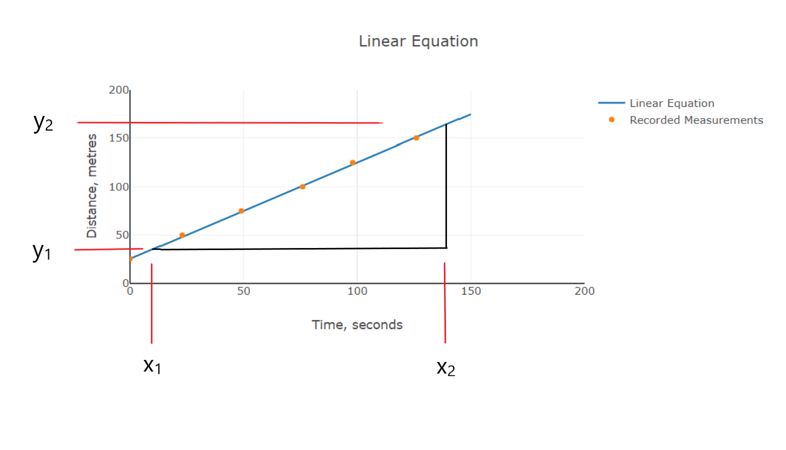
If you remember the linear equation [1] is: \[y = mx+c \] Where m is the gradient and c is the y intercept see the picture below:

Linear Equation drawn on a Graph

Therefore differentiating the linear equation:

\[y = mx^1 + c\] \[ \frac{dy}{dx} = m\]

Differentiating a constant term cancels it out so therefore 'c' the y intercept term disappears and you are left with the gradient term m as you would expect as the gradient is the rate of change of y with respect to x. If you differentiate a quadratic equation you will end a with a linear equation as shown below:

\[y = x^2 + 7x + 12\] \[ \frac{dy}{dx} = 2x + 7\]

Differentiation has many applications but one geometry defining use especially if you trying to get a curve to fit a specific line is it will tell you where the turning points are. At a turning point the rate of change is zero as at that point the curve is parallel to x-axis of the graph.

\[ \frac{dy}{dx} = 2x + 7 = 0\] \[x = \frac{-7}{2} = -3.5\] \[y = (-3.5)^2 + 7(-3.5) + 12\] \[= 12.25 -24.5 + 12 = -0.25 \]

This equation was used to demonstrate the quadratic equation in a earlier article [2], so therefore as its a quadratic there are two points where the curve would touch the x axis where y would be zero, they x = -4 and x = -3 if you remember \(y = (x + 4)(x + 3) = x^2 + 7x + 12\), its also simple to deduce that the curve touches the y axis at y = 12 when x =0. The graph below should demonstrate this all:

If you take a cubic equation as in the example below:

\[y = x^3 + 16x^2 + 75x + 108\] \[ \frac{dy}{dx} = 3x^2 + 32x + 75\]

As you can see differentiating a cubic equation gives a quadratic equation which is what you would expect as a cubic equation will have two turning points [3] and a quadratic equation has two values of x which will equate to zero representing the turning points. Similarly if you differentiate a quartic equation you will get cubic equation as a quartic equation has three points points, I think now you should see the general trend. Determining turning points is one of the many applications of differentiation, of course turning points tell you where you rate of change is zero which if you are looking at estimating maximum or minimum performance such as for aircraft this is very useful. The maximum aerodynamic performance of an aircraft can be determined using differentiation [4]. In later articles we at other ways you use differeniation, but the Stroud textbooks can also give you more information if need it quickly [5],[6].

Below gives a table of derivatives for various other common mathematical functions such a trignometry functions, etc. Derivative is the term used to describe the expression after you have differentiated the original mathematical expression. This article only serves as introduction of differential calculus, later articles will look at intergration calculus which is more or less the opposite of differentiation and more advanced differential techniques such as numerical methods. Calculus is the term used to refer to both differentiation and intergration collectively, further derivatives for various mathematical expressions can also be found in the Stroud textbooks [5], [6]. As an action point you could try differentiating the remaining polynomial equations which were not done in the this article from the previous article on polynomials [3]. If you feeling confident you could also derive the expressions for the aerodynamic ratios from the drag polar equation as discussed in an earlier article[4].

\(y = f(x)\)	\(\frac{d}{dx} f(x) = f'(x)\)
\(x^n\)	\(nx^{n-1}\)
\(e^x\)	\(e^{x}\)
\(ln(x)\)	\(\frac{1}{x}\)
\(sin(x)\)	\(cos(x)\)
\(cos(x)\)	\(-sin(x)\)
\(tan(x)\)	\(sec^2(x) = \frac{1}{cos^2(x)}= 1 +tan^2(x)\)

Please leave a comment on my facebook page or via email and let me know if you found this blog article useful and if you would like to see more on this topic. Most of my blog articles are on:

Mathematics
Helicopters
Woodworking and Boatbuilding

If there is one or more of these topics that you are specifically interested in please also let me know in your comments this will help me to write blog articles that are more helpful.

References:

[1] http://www.eiteog.com/EiteogBLOG/No15EiteogBlogLinear.html

[2] http://www.eiteog.com/EiteogBLOG/No34EiteogBlogQuadratic.html

[3] http://www.eiteog.com/EiteogBLOG/No37EiteogBlogPoly.html

[4] http://www.eiteog.com/EiteogBLOG/No46EiteogBlogRatios.html

[5] Engineering Mathematics, K. A. Stroud, Fourth Edition, 1995, Macmillan

[6] Further Engineering Mathematics, K. A. Stroud, Fourth Edition, 1996, Palgrave Macmillan

Disclaimer: Eiteog makes every effort to provide information which is as accurate as possible. Eiteog will not be responsible for any liability, loss or risk incurred as a result of the use and application of information on its website or in its products. None of the information on Eiteog's website or in its products supersedes any information contained in documents or procedures issued by relevant aviation authorities, manufacturers, flight schools or the operators of aircraft, UAVs.