
\[ \]
\[ \]
\[ \]
Issue No 15, 16 January 2023
By: Anthony O. Ives
The linear equation is a fundamental mathematical equation and concept. In reality most people use this concept all the time without knowing it when they estimate something based on an average value. The linear equation and linear relationship is simple to solve hence why in mathematics this terminology is used for any equation that has a solution. Unsolvable expressions are often referred to as non-linear, the Navier-Stokes equations (complicated equations which give a complete description of fluid mechanics, a future article will discuss them in more detail) are often referred to as non-linear. Ideally in mathematics various methods are applied to reduce complex relationships down to a principle linear equation but this is not always possible. The gradient is very easy to determine from a linear equation. The gradient often represents the rate of change between the two variables of the linear equation.
If one variable say 'y' depends on another variable say 'x' then 'y' is function of 'x'. 'y' is the general mathematical notation for a dependent variable as it dependents on 'x'. 'x' is therefore the general mathematical notation for independent variable. The following expression gives general mathematical notation that 'y' is dependent on 'x' but their relationship is not known:
y = f(x)
Sometimes you assume a relationship and use statistical or experimental results to prove the relationship is true. In case we obvious going to assume the linear equation which in its simplest form would be as below:
y=mx
Where 'm' is the gradient in this equation assumes that when 'y' is zero, 'x' is zero which may not always be the case. In reality 'y' may be equal to some arbitrary value 'c' when 'x' is zero hence a more general form of the linear equation is as follows:
y=mx+c
The notation 'c' is chosen to represent that this value is a constant, its also known as the y-intercept as its the point on graph where the graphically representation of the linear equation intercepts the y-axis. The linear equation gives a straight line when plotted on a graph which will be demonstrated later in this article. The notation 'y' and 'x' is used to generally represent any two variables that are related to one and other, so they were introduced here so you become familiar with what they mean. However, an example will give a better picture of how the linear equation is used. So left use time (t) as the 'x' variable and distance (s) as the 'y' variable therefore the linear equation would look like this:
s=vt
Where v is velocity which is of course the gradient 'm' as it represents the rate of change of distance (s) with time (t). Just to illustrate the y-intercept (c) it may be the case that time is measured from an offset distance (s0) which would then make the linear equation look this:
s = vt+s0
Where s0 is the y intercept value 'c'. To further demonstrate the usefulness of the linear equation and how to obtain a gradient from experimental results we will use example. I am going to use swimming as an example as enjoy swimming when I have free time. So say I want to determine my swim speed by getting my friend to time my swim laps or lengths so when I complete each lap my friend records the time. To demonstrate the y-intercept concept she will not start the stopwatch on the first lap to allow me to warm up. I will be using a 25 metre (m) pool I am estimating it will take me 25 seconds (s) to complete each length which is a speed of 1 metre per second. I am going to do 6 lengths including the warm up length which is 150m. Below gives a table of the times my friend has recorded and those I have estimated using the linear equation:
| Lap No | Distance (s)/m | Estimated Time (t)/s | Recorded Time (t)/s |
|---|---|---|---|
| 1 | 25 | 25 | 23 |
| 2 | 50 | 50 | 49 |
| 3 | 75 | 75 | 76 |
| 4 | 100 | 100 | 98 |
| 5 | 125 | 125 | 126 |
| 6 | 150 | 150 | 153 |
Normally the dependent variable (in this case distance, s) is measured at set intervals of the independent variable (in this case time, t). However, this was not possible for this scenario and does not really matter as long as you so always measure the most accurate way possible. For this scenario time can be measured more accurately for set intervals of distance, for other scenarios the reverse may be the better option and usually prefered way if you have a choice. The below graph shows the linear equation plotted as a solid line with the recorded measurements plotted as discrete markers:
You can determine the gradient by plotting your experimental results on a graph similar to what was does in the above graph. Plotting on graph obivously can be done with a computer program such as MS Excel but you can also do it manually using graph paper. The horizontal is usually called the x-axis as it represents the independent variable, the vertical axis is usually called the y-axis as it represents the dependent variable. To plot the points you would:
First select the value of the independent varable on the x-axis.
Then follow the grid line perpendicular to x-axis until it you reach the corresponding value of the dependent value on the y-axis.
Complete the above two steps for all the points.
Once you have plotted all the points you can draw a line of best fit using a ruler, line should be as close to all the points as possible.
From the line of best you can determine the gradient of the equation using trigonometry principles, see Ref[1]. Using the following steps should end of with a triangle:
Draw a line parallel to the y-axis from the further end of the best fit line the length of this line represents the opposite side on right angle triangle.
Draw a line parallel to the x-axis from the point the best fit line intercepts the y-axis the length of this line represents the adjacent side on right angle triangle.
The gradient is ratio of opposite over adjacent which is the same as tan(θ), see Ref[1] for more details
The below diagram should illustrate this:
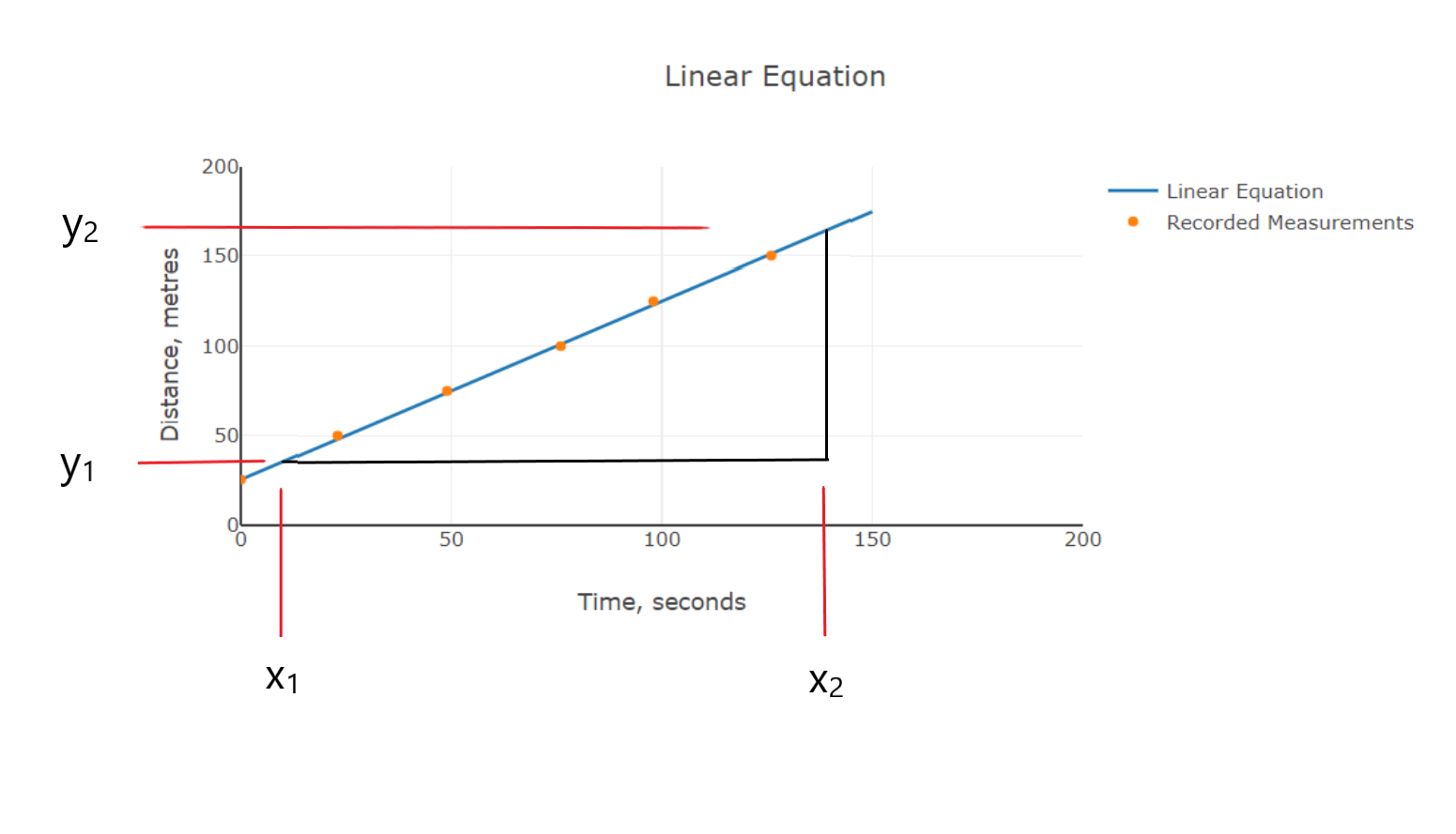
The gradient can also worked using the following formulae:
\[m=\frac{y_2-y_1}{x_2-x_1} \]
Where x2 is the larger value on the x-axis, y2 is the value on the y-axis corresponding to x2, x1 is the smaller value on the x-axis, y1 is the value on the y-axis corresponding to x1. You can use a triange of any size as long as the best fit line forms part of the hypotenuse side (see Ref [1] for an explanation) of the triangle, the bigger the triangle the more accurately the gradient can be caluclated.
Modern computer programs such as MS Excel use a method called 'Least Squares' to accurately calculate a line of best fit and work out a gradient from a set of points, a future article will discuss this method in more detail however further information can be found on curve fitting in Ref[2] and [3].
Just out of interest in the pool that I swim in you need to able to swim 25 seconds in 25 metres to use the fast lane. 30 seconds in 25 metres to use the medium lane and 40 seconds in 25 metres to use the recreation lane. Ref [4] mentions the swim records were set by first by an American swimmer Matt Bondi at 22 seconds in 50 metres and then broken by a Russian swimmer Alexander Popov at 21.8 seconds for the same distance in 1992. That works out at 11 seconds for 25 metres, since then the record may have been broken again but this gives you an idea of typical top speeds of a human swimmer. Apparently a polar bear can do in 9 seconds approximately, maybe less time so I will not even mention things likes sharks, etc. Ref [4] gives a good guide on how to improve your swimming by making it more efficient concentrating on streamlining and using less energy to swim faster. Ref [4] is also interesting in that discusses how swim technique can be compared to boat hull design.
Please leave a comment on my facebook page or via email and let me know if you found this blog article useful and if you would like to see more on this topic. Most of my blog articles are on:
Mathematics
Helicopters
Woodworking and Boatbuilding
If there is one or more of these topics that you are specifically interested in please also let me know in your comments this will help me to write blog articles that are more helpful.
References:
[1] http://www.eiteog.com/EiteogBLOG/No12EiteogBlogTrig.html
[2] Engineering Mathematics, K. A. Stroud, Fourth Edition, 1995, Macmillan
[3] Probability and Statistics in Engineering, William W. Hines, Douglas M. Montgomery, David M. Goldman, Connie M. Borror, Fourth Edition, 2003, Wiley
[4] 'Total immersion: The revolutionary way to swim better, faster and easier', Terry Laughlin, John Delves, 2004, Fireside
![]()


Disclaimer: Eiteog makes every effort to provide information which is as accurate as possible. Eiteog will not be responsible for any liability, loss or risk incurred as a result of the use and application of information on its website or in its products. None of the information on Eiteog's website or in its products supersedes any information contained in documents or procedures issued by relevant aviation authorities, manufacturers, flight schools or the operators of aircraft, UAVs.
For any inquires contact: [email protected] copyright © Eiteog 2022